Getting started with timeseries data augmentation

Data augmentation is a critical component in modern machine learning practice due to its benefits for model accuracy, generalizability, and robustness to adversarial examples. Elucidating the precise mechanisms by which this occurs is a currently active area of research, but a simplified explanation of the current proposals might look like this:

1. adding noise to the feature space is form of regularization; and,
2. adding examples with similar semantic value but different features forces a model to learn invariant representations of those semantics.

It's pretty intuitive to reason about transforms which trigger these mechanisms in fields like computer vision, since we all have personal experience with photography and images. For example, you can imagine mild blurring or dust on the lens as strategies for triggering that first mechanism, and flipping an image horizontally (from left to right) as a strategy for triggering the second mechanism. And indeed, things like flipping, cropping, rotating, and blurring an image are common image data augmentation strategies.

Timeseries data seems less intuitive than images in the sense we are using it here: even though we all have daily experience with time, not all of us look at heterogeneous collections of timeseries data as a part of our nonprofessional lives. Let's take a single example to make this a bit more clear. For an timeseries of recorded human speech (i.e. the actual audio), shifting the frequencies around a little bit could be seen as a semantics-preserving transform -- we are making the voice higher or lower pitched, but the vowels and consonants remain the same. For a timeseries of recorded temperatures, shifting the frequencies around a little bit would be an extreme form of noise -- instead of the peak temperatures from summer to summer being 12 months apart, they might be 11 or 13.

To give ourselves a better idea about how to use timeseries data augmentations, we can look at a few operations performed on some real world data. Let's use Apple's daily closing stock price from the last few years.

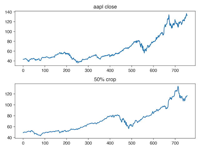
"Classical" timeseries methods make some assumptions about the data generating process, which, among other things, includes stationarity and self-similarity. A lot of timeseries data preprocessing steps are concerned with coercing real distributions into fitting these assumptions, at least in a weak sense. If we assume that this assumption holds in our data, one semantics-preserving transform we might apply is random cropping. In the same way that cropping a part of an image and resizing it to match the original works for photographs as long as part of the object of interest is still in the crop, we can select a subset of our series as long as it has enough of the signal left to still capture the dynamics that we care about.

Here is a before-and-after of using crop_and_stretch from niacin on our stock data. Note the strong self-similarity between the full series, and a random crop of that series:

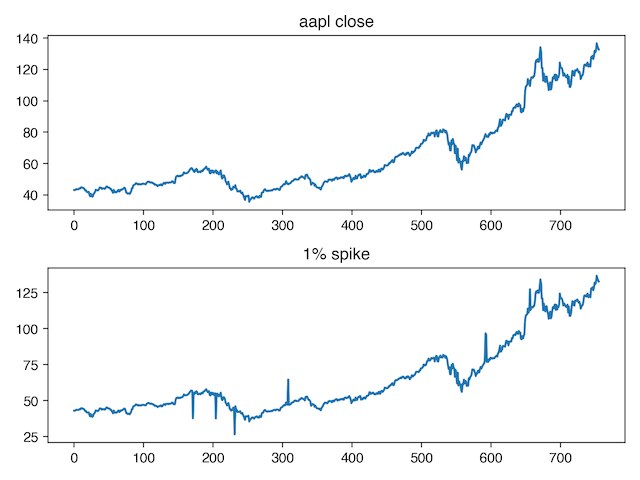
Now let's look at regularization. We might want to end up with a model that is robust to anomalous spikes in the timeseries. To encourage the model to learn this behavior, we can add spikes to the augmented data during training (spike magnitude is exaggerated to make them easier to see).

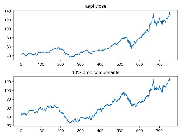
Or, we might a model that pays attention to both high frequency changes in the input, and low frequency changes in the input. To do this, we can convert our series to the fequency domain, then randomly drop components (you can think about this as a form of "data dropout").

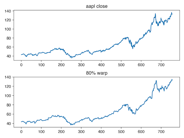
If we want our model to generalize across small disruptions in event time, we can add random warping (this one is a bit harder to see -- focus on the dip around x=580) which keeps the values in the same order, but changes how much time occurs between each recorded value.

For more examples of timeseries augmentation transforms, check out niacin's user guide.

timeseries augmentation python niacin